
Shortest Path Problem: Dijkstra’s Algorithm Explained with Real-World Scenarios
Introduction
Imagine you are using Google Maps to travel from your university to a nearby restaurant. Within seconds, the app calculates the shortest route, avoids traffic, and guides you efficiently.
Have you ever wondered how it finds the best path so quickly?
The answer often lies in Dijkstra’s Algorithm, one of the most important graph algorithms in computer science.
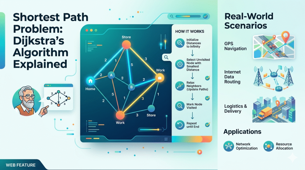
Dijkstra’s Algorithm solves the Shortest Path Problem, helping computers determine the minimum distance between two points in a network.
This algorithm is widely used in:
- GPS Navigation Systems
- Internet Routing
- Social Network Analysis
- Robotics
- Delivery Route Optimization
- Gaming Pathfinding
In this blog, we’ll break down Dijkstra’s Algorithm in a simple, human-friendly way using real-world scenarios.
What is the Shortest Path Problem?
The Shortest Path Problem asks:
What is the shortest possible route between two nodes in a weighted graph?
A graph consists of:
- Vertices (Nodes) → Locations
- Edges → Connections between locations
- Weights → Distance, time, or cost
Real-Life Example
Suppose a student wants to travel from Home to COMSATS University.
Possible routes:
| Route | Distance |
|---|---|
| Home → Mall → University | 12 km |
| Home → Park → University | 9 km |
| Home → Market → University | 15 km |
The goal is to find the minimum distance path.
This is exactly what Dijkstra’s Algorithm does.
What is Dijkstra’s Algorithm?
Dijkstra’s Algorithm is a graph search algorithm used to find the shortest path from a source node to all other nodes in a weighted graph.
It was developed by Edsger W. Dijkstra in 1956.
The algorithm works on graphs with:
✅ Non-negative edge weights
❌ Does not work correctly with negative weights

Real-World Scenario: Food Delivery System
Let’s say a food delivery rider must deliver an order from a restaurant to a customer.
Possible roads:
- Restaurant → Market = 4 min
- Restaurant → Signal = 2 min
- Market → Customer = 5 min
- Signal → Customer = 3 min
The system must choose the fastest route.
Dijkstra’s Algorithm calculates:
Restaurant → Signal → Customer = 5 min
instead of
Restaurant → Market → Customer = 9 min
This saves time and fuel.
That’s how apps like Uber Eats and Foodpanda optimize deliveries.
How Dijkstra’s Algorithm Works
The algorithm follows these steps:
Step 1: Assign Initial Distances
- Source node = 0
- All other nodes = ∞
Step 2: Visit the Nearest Unvisited Node
Choose the node with the smallest known distance.
Step 3: Update Neighbor Distances
If a shorter path is found through the current node, update it.
Step 4: Mark Node as Visited
Once processed, it is finalized.
Step 5: Repeat Until All Nodes Are Processed

Find shortest path from A to F
To find the shortest path from the starting vertex A to all other vertices using Dijkstra’s Algorithm, we maintain a list of shortest known distances from A, updating them step-by-step.
Initial Setup
-
Distance to starting vertex A: 0
-
Distance to all other vertices (B, C, D, E, F): (Infinity)
-
Visited set: (Empty)
Step-by-Step Execution
Step 1: Select vertex A (Current minimum distance = $0$)
-
Mark A as visited.
-
Update distances to unvisited neighbors of A:
-
To B: min(infty, 0 + 4) = 4 via A
-
To C: min(infty, 0 + 5) = 5 via A
- Current Distance Table:
-
| Vertex | Distance | Pre. Vertex | Status |
| A | 0 | – | Visited |
| B | 4 | A | Unvisited |
| C | 5 | A | Unvisited |
| D | infty | – | Unvisited |
| E | infty | – | Unvisited |
| F | infty | – | Unvisited |
Step 2: Select vertex B (Current minimum unvisited distance = 4)
-
Mark B as visited.
-
Update distances to unvisited neighbors of B:
-
To C: min(5, 4 + 11) = 5 (No change, 5 is shorter than 15)
-
To D: min(infty, 4 + 9) = 13 via B
-
To E: min(infty, 4 + 7) = 11 via B
-
-
Current Distance Table:
| Vertex | Distance | Pre. Vertex | Status |
| A | 0 | – | Visited |
| B | 4 | A | Visited |
| C | 5 | A | Unvisited |
| D | 13 | B | Unvisited |
| E | 11 | B | Unvisited |
| F | infty | – | Unvisited |
Step 3: Select vertex C (Current minimum unvisited distance = 5)
-
Mark C as visited.
-
Update distances to unvisited neighbors of C:
-
To E: min(11, 5 + 3) = 8 via C (Updated since 8 is shorter than 11)
-
-
Current Distance Table:
| Vertex | Distance | Pre. Vertex | Status |
| A | 0 | – | Visited |
| B | 4 | A | Visited |
| C | 5 | A | Visited |
| D | 13 | B | Unvisited |
| E | 8 | C | Unvisited |
| F | infty | – | Unvisited |
Step 4: Select vertex E (Current minimum unvisited distance = $8$)
-
Mark E as visited.
-
Update distances to unvisited neighbors of E:
-
To D: min(13, 8 + 13) = 13 (No change)
-
To F: min(infty, 8 + 6) = 14 via E
-
-
Current Distance Table:
| Vertex | Distance | Pre. Vertex | Status |
| A | 0 | – | Visited |
| B | 4 | A | Visited |
| C | 5 | A | Visited |
| D | 13 | B | Unvisited |
| E | 8 | C | Visited |
| F | 14 | E | Unvisited |
Step 5: Select vertex D (Current minimum unvisited distance = 13)
-
Mark D as visited.
-
Update distances to unvisited neighbors of D:
-
To F: min(14, 13 + 2) = 15 (No change, 14 is shorter than 15)
-
-
Current Distance Table:
| Vertex | Distance | Prev. Vertex | Status |
| A | 0 | – | Visited |
| B | 4 | A | Visited |
| C | 5 | A | Visited |
| D | 13 | B | Visited |
| E | 8 | C | Visited |
| F | 14 | E | Unvisited |
Step 6: Select vertex F (Remaining vertex = 14)
-
Mark F as visited. Algorithm terminates.
Final Summary Table
By tracking the “Previous Vertex” backwards, we can extract the shortest path from A to every destination:
| Destination Vertex | Shortest Distance | Shortest Path |
| A | 0 | A |
| B | 4 | A —–> B |
| C | 5 | A —–> C |
| D | 13 | A —–> B —–> D |
| E | 8 | A —–> C —–> E |
| F | 14 | A —–> C —–> E —–> F |
Pseudocode of Dijkstra’s Algorithm
1. Set distance[source] = 0
2. Set all other distances = ∞
3. Add all nodes to priority queue
4. While queue is not empty:
Extract node with minimum distance
For each neighbor:
newDist = currentDist + edgeWeight
If newDist < known distance:
Update distance
Generic C++ implementation of Dijkstra’s Algorithm
#include <iostream>
#include <vector>
#include <queue>
#include <climits>

using namespace std;

void dijkstra(int source, vector<vector<pair<int, int>>> &graph, int vertices)
{
    // Step 1 & 2: Initialize distances
    vector<int> distance(vertices, INT_MAX);
    distance[source] = 0;

    // Step 3: Priority Queue
    priority_queue<pair<int, int>,
            vector<pair<int, int>>,
            greater<pair<int, int>>> pq;

    pq.push({0, source});

    // Step 4: Process until queue is empty
    while (!pq.empty())
    {
        int currentDist = pq.top().first;
        int currentNode = pq.top().second;
        pq.pop();

        // Visit all neighbors
        for (auto neighbor : graph[currentNode])
        {
            int nextNode = neighbor.first;
            int edgeWeight = neighbor.second;

            int newDist = currentDist + edgeWeight;

            // Update distance if shorter path found
            if (newDist < distance[nextNode])
            {
                distance[nextNode] = newDist;
                pq.push({newDist, nextNode});
            }
        }
    }

    // Print shortest distances
    cout << "Shortest distances from source node " << source << ":\n";

    for (int i = 0; i < vertices; i++)
    {
        cout << "Node " << i << " : ";

        if (distance[i] == INT_MAX)
            cout << "Infinity";
        else
            cout << distance[i];

        cout << endl;
    }
}

int main()
{
    int vertices = 5;

    vector<vector<pair<int, int>>> graph(vertices);

    // Add edges
    graph[0].push_back({1, 4});
    graph[0].push_back({2, 1});

    graph[1].push_back({3, 1});
    graph[2].push_back({1, 2});
    graph[2].push_back({3, 5});

    graph[3].push_back({4, 3});

    int source = 0;

    dijkstra(source, graph, vertices);

    return 0;
}
Time Complexity
The efficiency depends on implementation.
Using Array
O(V²)
Using Priority Queue
O((V + E) log V)
This makes it efficient for large-scale applications.
Real-Life Applications of Dijkstra’s Algorithm
1. GPS Navigation
Apps like Google Maps calculate shortest driving routes.
Scenario:
A student traveling from Sahiwal to Lahore gets the fastest route.
2. Network Routing
Internet packets travel through shortest paths.
Used in routing protocols like OSPF.
Scenario:
When opening a website, data chooses the fastest route across servers.
3. Ride-Hailing Apps
Apps like Uber assign nearest drivers.
Scenario:
The app finds the driver who can reach the passenger quickest.
4. Robotics
Robots navigate efficiently.
Scenario:
A warehouse robot finds the shortest path to retrieve products.
5. Social Networks
Finding shortest connections between people.
Scenario:
Determining mutual friend connections in Meta platforms.
Advantages of Dijkstra’s Algorithm
✅ Simple to understand
✅ Efficient for non-negative graphs
✅ Widely applicable
✅ Guarantees shortest path
Limitations
Cannot handle negative edge weights
Can become slower for massive dense graphs
For graphs with negative weights, use Bellman-Ford Algorithm instead.
Dijkstra vs Bellman-Ford
| Feature | Dijkstra | Bellman-Ford |
|---|---|---|
| Negative Weights | No | Yes |
| Speed | Faster | Slower |
| Complexity | O(V²) | O(VE) |
Conclusion
Dijkstra’s Algorithm is far more than just a classroom topic.
It powers:
- Navigation apps
- Delivery services
- Internet communication
- Smart transportation systems
By understanding this algorithm, students gain practical skills for solving real-world optimization problems.
The next time your map app finds the fastest route, remember:
A graph algorithm is working behind the scenes — and there’s a good chance it’s Dijkstra’s Algorithm.

 Explained with Real-Life Example | Step-by-Step Guide")
 Using Kruskal Algorithm Explained with Real-Life Example | Step-by-Step Guide")
