
Graph Representation by Matrix, Graph Traversals, and Dijkstra Algorithm Explained with Practical Examples
Introduction
Graphs are among the most powerful and widely used data structures in computer science. From social media connections to GPS navigation systems, graphs help model relationships between objects efficiently.
Imagine opening Google Maps and searching for the shortest route to your destination. Behind the scenes, graph algorithms work continuously to determine the best path.
In this blog, we will explore:
- Graph representation using matrix
- Graph traversal techniques
- Dijkstra’s shortest path algorithm
- Practical examples with C++ code
By the end, you’ll have a solid understanding of how graphs work and how they solve real-world problems.
What is a Graph Data Structure?
A Graph is a non-linear data structure consisting of:
- Vertices (Nodes) → Represent entities
- Edges → Represent connections between entities
A graph can be:
1. Directed Graph
Edges have direction.
Example: Instagram follow system
If A follows B, it does not mean B follows A.
2. Undirected Graph
Edges have no direction.
Example: Facebook friendship
If A is a friend of B, B is automatically a friend of A.
Real-Life Example of Graph
Consider a university campus navigation system.
Buildings are represented as vertices:
- Library
- Cafeteria
- Lab
- Admin Block
Roads connecting them are edges.
The system uses graph algorithms to find the shortest path between two buildings.
Graph Representation by Matrix
A graph can be represented in multiple ways, but one common method is the Adjacency Matrix.
What is an Adjacency Matrix?
An adjacency matrix is a 2D array where:
- Rows represent source vertices
- Columns represent destination vertices
If there is an edge between two vertices:
- Put 1 (or weight)
- Otherwise put 0
Example Graph
Suppose we have 4 vertices:
A, B, C, D
Connections:
- A → B
- A → C
- B → D
- C → D
Adjacency Matrix
| A | B | C | D | |
|---|---|---|---|---|
| A | 0 | 1 | 1 | 0 |
| B | 0 | 0 | 0 | 1 |
| C | 0 | 0 | 0 | 1 |
| D | 0 | 0 | 0 | 0 |
C++ Implementation of Adjacency Matrix
#include <iostream>
using namespace std;

int main() {
    int graph[4][4] = {
        {0,1,1,0},
        {0,0,0,1},
        {0,0,0,1},
        {0,0,0,0}
    };

    cout << "Adjacency Matrix:" << endl;

    for(int i=0; i<4; i++) {
        for(int j=0; j<4; j++) {
            cout << graph[i][j] << " ";
        }
        cout << endl;
    }

    return 0;
}
Output:
0 1 1 0
0 0 0 1
0 0 0 1
0 0 0 0
Graph Traversals
Graph traversal means visiting every node of a graph systematically.
There are two main traversal techniques:
- Breadth First Search (BFS)
- Depth First Search (DFS)
Lesson 23: Graph Traversal Techniques Explained: BFS and DFS with Real-Time Examples
Breadth First Search (BFS)
BFS visits nodes level by level.
It uses a Queue data structure.
Practical Example of BFS
Suppose a university wants to send notifications to all students.
The notification spreads:
- First to CRs
- Then class representatives inform students
This level-wise spreading resembles BFS.
BFS Working
For graph:
A
/ \
B C
\ /
D
Traversal:
A → B → C → D
C++ Code for BFS
#include <iostream>
#include <queue>
using namespace std;

void BFS(int graph[4][4], int start) {
    bool visited[4] = {false};
    queue<int> q;

    visited[start] = true;
    q.push(start);

    while(!q.empty()) {
        int node = q.front();
        q.pop();

        cout << node << " ";

        for(int i=0; i<4; i++) {
            if(graph[node][i] && !visited[i]) {
                visited[i] = true;
                q.push(i);
            }
        }
    }
}

int main() {
    int graph[4][4] = {
        {0,1,1,0},
        {0,0,0,1},
        {0,0,0,1},
        {0,0,0,0}
    };

    BFS(graph, 0);

    return 0;
}
Depth First Search (DFS)
DFS explores as deep as possible before backtracking.
It uses a Stack (or recursion).
Practical Example of DFS
Think of searching files in nested folders.
You open one folder, then subfolder, then deeper subfolder before returning.
That is DFS.
DFS Traversal
For the same graph:
A → B → D → C
C++ Code for DFS
#include <iostream>
using namespace std;

void DFS(int graph[4][4], bool visited[], int node) {
    visited[node] = true;
    cout << node << " ";

    for(int i=0; i<4; i++) {
        if(graph[node][i] && !visited[i]) {
            DFS(graph, visited, i);
        }
    }
}

int main() {
    int graph[4][4] = {
        {0,1,1,0},
        {0,0,0,1},
        {0,0,0,1},
        {0,0,0,0}
    };

    bool visited[4] = {false};

    DFS(graph, visited, 0);

    return 0;
}
Lesson 24: Shortest Path Problem: Dijkstra’s Algorithm Explained with Real-World Scenarios
Dijkstra’s Algorithm
Dijkstra’s Algorithm finds the shortest path between nodes in a weighted graph.
It is widely used in:
- GPS Navigation
- Network Routing
- Airline Route Optimization
- Robotics
Real-Life Practical Example
Suppose a student wants to reach the university from home.
Possible routes:
| Route | Distance |
|---|---|
| Home → Road A → University | 10 km |
| Home → Road B → University | 7 km |
| Home → Road C → University | 12 km |
Dijkstra’s Algorithm finds:
Shortest Path = Road B (7 km)
How Dijkstra Works
Step 1
Set source distance = 0
Step 2
Set all others = Infinity
Step 3
Select nearest unvisited node
Step 4
Update neighboring distances
Step 5
Repeat until all nodes are processed
C++ Implementation of Dijkstra Algorithm
#include <iostream>
#include <climits>
using namespace std;

#define V 5

int minDistance(int dist[], bool visited[]) {
    int min = INT_MAX, min_index;

    for(int v=0; v<V; v++) {
        if(!visited[v] && dist[v] <= min) {
            min = dist[v];
            min_index = v;
        }
    }

    return min_index;
}

void dijkstra(int graph[V][V], int src) {
    int dist[V];
    bool visited[V];

    for(int i=0; i<V; i++) {
        dist[i] = INT_MAX;
        visited[i] = false;
    }

    dist[src] = 0;

    for(int count=0; count<V-1; count++) {
        int u = minDistance(dist, visited);
        visited[u] = true;

        for(int v=0; v<V; v++) {
            if(!visited[v] && graph[u][v] &&
                    dist[u] != INT_MAX &&
                    dist[u] + graph[u][v] < dist[v]) {
                dist[v] = dist[u] + graph[u][v];
            }
        }
    }

    cout << "Vertex Distance from Source\n";
    for(int i=0; i<V; i++)
        cout << i << "\t" << dist[i] << endl;
}

int main() {
    int graph[V][V] = {
        {0,10,0,30,100},
        {10,0,50,0,0},
        {0,50,0,20,10},
        {30,0,20,0,60},
        {100,0,10,60,0}
    };

    dijkstra(graph, 0);

    return 0;
}
Output:
Vertex Distance from Source
0 0
1 10
2 50
3 30
4 60
Why Graph Algorithms Matter
Graph algorithms are essential in modern computing.
They power:
Social Networks
Friend suggestions on platforms
Search Engines
Ranking web pages
Navigation Systems
Finding shortest routes
Computer Networks
Efficient packet transfer
AI and Machine Learning
Knowledge graphs
Activity Outcomes
After completing this lab, students will be able to:
✅ Understand Graph Data Structure
✅ Represent graphs using matrix
✅ Implement BFS traversal
✅ Implement DFS traversal
✅ Apply Dijkstra Algorithm
✅ Solve shortest path problems
onclusion
Graph data structures are fundamental for solving real-world connectivity and optimization problems.
Understanding:
- Graph representation by matrix
- BFS
- DFS
- Dijkstra’s Algorithm
builds a strong foundation for advanced topics like:
- Artificial Intelligence
- Networking
- Competitive Programming
- Machine Learning
Mastering these concepts will significantly improve your problem-solving skills as a programmer.
Activity 1:
Implements the Graph data structure by Adjacency Matrix.
Consider the following Graph:
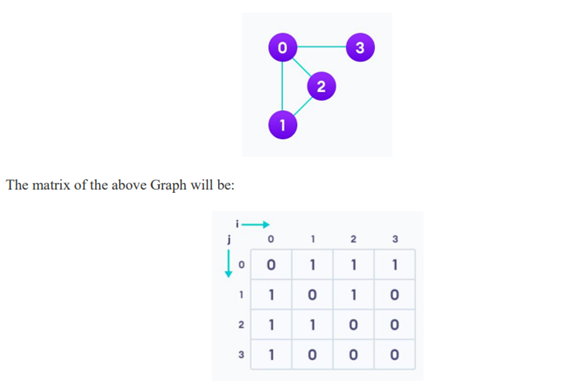
C++ code to implement the graph using an Adjacency Matrix exactly according to the graph shown in your activity.
C++ Code: Graph Implementation using Adjacency Matrix
#include <iostream>
using namespace std;

int main() {
    const int vertices = 4;

    // Adjacency Matrix based on given graph
    int graph[vertices][vertices] = {
        {0, 1, 1, 1},
        {1, 0, 1, 0},
        {1, 1, 0, 0},
        {1, 0, 0, 0}
    };

    cout << "Adjacency Matrix Representation of Graph:\n\n";

    // Display column labels
    cout << "   ";
    for(int i = 0; i < vertices; i++) {
        cout << i << " ";
    }
    cout << endl;

    // Display matrix
    for(int i = 0; i < vertices; i++) {
        cout << i << "  ";
        for(int j = 0; j < vertices; j++) {
            cout << graph[i][j] << " ";
        }
        cout << endl;
    }

    return 0;
}
Explanation
This matrix represents the connections:
- 0 → 1, 2, 3
- 1 → 0, 2
- 2 → 0, 1
- 3 → 0
Since the graph is undirected, the matrix is symmetric, meaning:
If vertex i is connected to vertex j, then vertex j is also connected to vertex i.
Activity 2:
Implement the Graph by Adjacency List.
C++ code to implement the same graph using an Adjacency List representation.
#include <iostream>
#include <vector>
using namespace std;

int main() {
    const int vertices = 4;

    // Adjacency List
    vector<int> graph[vertices];

    // Adding edges according to given graph
    graph[0].push_back(1);
    graph[0].push_back(2);
    graph[0].push_back(3);

    graph[1].push_back(0);
    graph[1].push_back(2);

    graph[2].push_back(0);
    graph[2].push_back(1);

    graph[3].push_back(0);

    // Display adjacency list
    cout << "Adjacency List Representation of Graph:\n\n";

    for(int i = 0; i < vertices; i++) {
        cout << i << " -> ";
        for(int j = 0; j < graph[i].size(); j++) {
            cout << graph[i][j] << " ";
        }
        cout << endl;
    }

    return 0;
}
Output:
Adjacency List Representation of Graph:
0 -> 1 2 3
1 -> 0 2
2 -> 0 1
3 -> 0
Explanation
The graph connections are stored as lists:
- 0 → 1, 2, 3
- 1 → 0, 2
- 2 → 0, 1
- 3 → 0
Why use Adjacency List?
Adjacency List is useful when the graph has fewer edges because it:
✅ Uses less memory
✅ Faster for traversing neighbors
✅ Efficient for sparse graphs
Graded Task: Real-Time Scenario on Graph Representation, Traversals, and Dijkstra Algorithm
Scenario: Smart University Campus Navigation System
COMSATS University Islamabad plans to develop a Smart Campus Navigation System for newly admitted students and visitors.
The university campus has multiple important locations connected through roads:
- A = Main Gate
- B = Administration Block
- C = Library
- D = Computer Science Department
- E = Cafeteria
- F = Hostel
The roads between these locations have specific distances (in meters).
Campus Road Network
| From | To | Distance |
|---|---|---|
| A | B | 4 |
| A | C | 2 |
| B | D | 5 |
| B | E | 10 |
| C | D | 8 |
| C | E | 3 |
| D | F | 6 |
| E | F | 2 |
Problem Statement
The university wants students to build a system that can:
- Represent the campus map using an Adjacency Matrix
- Traverse all locations using:
- Breadth First Search (BFS)
- Depth First Search (DFS)
- Find the shortest route from Main Gate (A) to Hostel (F) using Dijkstra’s Algorithm
Student Task (Graded Assignment)
Task 1: Graph Representation (5 Marks)
Construct the Adjacency Matrix for the campus road network.
Task 2: BFS Traversal (5 Marks)
Write a C++ program to perform Breadth First Search starting from Main Gate (A).
Expected Output Example:
A → B → C → D → E → F
Task 3: DFS Traversal (5 Marks)
Write a C++ program to perform Depth First Search starting from Main Gate (A).
Expected Output Example:
A → B → D → F → E → C
(Note: Output may vary depending on traversal order.)
Task 4: Dijkstra Algorithm (10 Marks)
Implement Dijkstra’s Algorithm to determine:
- Shortest path from Main Gate (A) to Hostel (F)
- Total minimum distance
Task 5: Analysis Question (5 Marks)
Answer the following:
Q1: Why is BFS more suitable for level-wise exploration?
Q2: Why does Dijkstra’s Algorithm provide an optimal solution?
Q3: What is the limitation of Adjacency Matrix representation?
Expected Real-Time Output
The system should display:
Shortest Path:
A → C → E → F
Minimum Distance:
7 meters

 Explained with Real-Life Example | Step-by-Step Guide")
 Using Kruskal Algorithm Explained with Real-Life Example | Step-by-Step Guide")
